RETIS in a 2D potential

In this example, you will explore a rare event with the Replica Exchange Transition Interface Sampling (RETIS) algorithm.

In this example, we will implement a new potential for PyRETIS and we will create three new order parameters which we will use to investigate a transition between two stable states in the potential. Using the RETIS algorithm, we will compute the rate constant for the transition between the two stable states.

This example is structured as follows:

Creating the potential function

We will consider a relatively simple 2D potential where a single particle is moving. The potential energy () is given by

where and gives the positions. The potential energy is shown in Fig. 25 below.

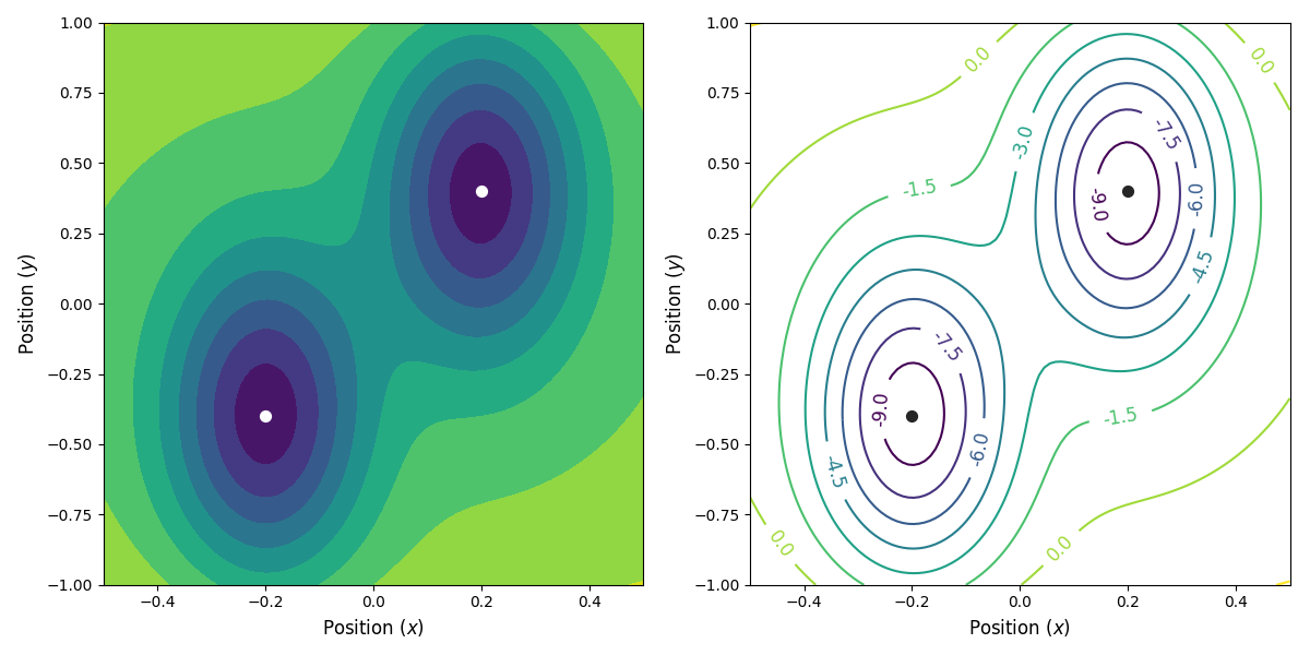
Fig. 25 The potential energy as a function of the position. We have two stable states, at (x, y) = (-0.2, -0.4) and (x, y) = (0.2, 0.4) (indicated with the circles), separated by a saddle point at (x, y) = (0, 0).

We begin by creating a new potential function to use with PyRETIS, see the user guide for a short introduction on how custom potential functions can be created. In short, we will now have to define a new class which calculates the potential energy and the corresponding force.

We begin by simply creating a new class for the new potential function. Here, we define the parameters our new potential should accept. We implement the potential slightly more general than the potential given above so that we can change the parameters more easily, if we wish to do so, later. The potential we will be implementing is given by:

where , , , , , , , and are potential parameters.

Next, we define a new method as part of our new potential class which will be responsible for calculating the potential energy and a method responsible for calculating the force. Finally, we add a method that will calculate both the potential and the force at the same time. The full Python code for the new potential class can be found below.

Show/hide the new potential class »

# -*- coding: utf-8 -*-
# Copyright (c) 2019, PyRETIS Development Team.
# Distributed under the LGPLv2.1+ License. See LICENSE for more info.
"""This is a 2D example potential."""
import logging
import numpy as np
from pyretis.forcefield.potential import PotentialFunction
logger = logging.getLogger(__name__)  # pylint: disable=invalid-name
logger.addHandler(logging.NullHandler())


class Hyst2D(PotentialFunction):
    r"""Hyst2D(PotentialFunction).

    This class defines a 2D dimensional potential with two
    stable states.
    The potential energy (:math:`V_\text{pot}`) is given by

    .. math::

       V_\text{pot}(x, y) = \gamma_1 (x^2 + y^2)^2 +
       \gamma_2 \exp(\alpha_1 (x - x_0)^2 + \alpha_2 (y - y_0)^2) +
       \gamma_3 \exp(\beta_1 (x + x_0)^2 + \beta_2(y + y_0)^2)

    where :math:`x` and :math:`y` gives the positions and :math:`\gamma_1`,
    :math:`\gamma_2`, :math:`\gamma_3`, :math:`\alpha_1`, :math:`\alpha_2`,
    :math:`\beta_1`, :math:`\beta_2`, :math:`x_0` and :math:`y_0` are
    potential parameters.

    Attributes
    ----------
    params : dict
        Contains the parameters. The keys are:

        * `gamma1`: The :math:`\gamma_1` parameter for the potential.
        * `gamma2`: The :math:`\gamma_2` parameter for the potential.
        * `gamma3`: The :math:`\gamma_3` parameter for the potential.
        * `alpha1`: The :math:`\alpha_1` parameter for the potential.
        * `alpha2`: The :math:`\alpha_2` parameter for the potential.
        * `beta1`: The :math:`\beta_1` parameter for the potential.
        * `beta2`: The :math:`\beta_2` parameter for the potential.
        * `x0`: The :math:`x_0` parameter for the potential.
        * `y0`: The :math:`y_0` parameter for the potential.

    """

    def __init__(self, desc='2D hysteresis'):
        """Set up the potential.

        Parameters
        ----------
        a : float, optional
            Parameter for the potential.
        b : float, optional
            Parameter for the potential.
        c : float, optional
            Parameter for the potential.
        desc : string, optional
            Description of the force field.

        """
        super().__init__(dim=2, desc=desc)
        self.params = {'gamma1': 0.0, 'gamma2': 0.0, 'gamma3': 0.0,
                       'alpha1': 0.0, 'alpha2': 0.0, 'beta1': 0.0,
                       'beta2': 0.0, 'x0': 0.0, 'y0': 0.0}

    def potential(self, system):
        """Evaluate the potential.

        Parameters
        ----------
        system : object like `System`
            The system we evaluate the potential for. Here, we
            make use of the positions only.

        Returns
        -------
        out : float
            The potential energy.

        """
        x = system.particles.pos[:, 0]  # pylint: disable=invalid-name
        y = system.particles.pos[:, 1]  # pylint: disable=invalid-name
        gam1 = self.params['gamma1']
        gam2 = self.params['gamma2']
        gam3 = self.params['gamma3']
        alf1 = self.params['alpha1']
        alf2 = self.params['alpha2']
        bet1 = self.params['beta1']
        bet2 = self.params['beta2']
        x_0 = self.params['x0']
        y_0 = self.params['y0']
        v_pot = (gam1 * (x**2 + y**2)**2 +
                 gam2 * np.exp(alf1 * (x - x_0)**2 + alf2 * (y - y_0)**2) +
                 gam3 * np.exp(bet1 * (x + x_0)**2 + bet2 * (y + y_0)**2))
        return v_pot.sum()

    def force(self, system):
        """Evaluate forces.

        Parameters
        ----------
        system : object like `System`
            The system we evaluate the potential for. Here, we
            make use of the positions only.

        Returns
        -------
        out[0] : numpy.array
            The calculated force.
        out[1] : numpy.array
            The virial, currently not implemented for this potential.

        """
        x = system.particles.pos[:, 0]  # pylint: disable=invalid-name
        y = system.particles.pos[:, 1]  # pylint: disable=invalid-name
        gam1 = self.params['gamma1']
        gam2 = self.params['gamma2']
        gam3 = self.params['gamma3']
        alf1 = self.params['alpha1']
        alf2 = self.params['alpha2']
        bet1 = self.params['beta1']
        bet2 = self.params['beta2']
        x_0 = self.params['x0']
        y_0 = self.params['y0']
        term = 4.0 * gam1 * (x**2 + y**2)
        exp1 = gam2 * np.exp(alf1 * (x - x_0)**2 + alf2 * (y - y_0)**2)
        exp2 = gam3 * np.exp(bet1 * (x + x_0)**2 + bet2 * (y + y_0)**2)
        forces = np.zeros_like(system.particles.pos)
        forces[:, 0] = -(x * term +
                         2.0 * alf1 * (x - x_0) * exp1 +
                         2.0 * bet1 * (x + x_0) * exp2)
        forces[:, 1] = -(y * term +
                         2.0 * alf2 * (y - y_0) * exp1 +
                         2.0 * bet2 * (y + y_0) * exp2)
        virial = np.zeros((self.dim, self.dim))  # just return zeros here
        return forces, virial

    def potential_and_force(self, system):
        """Evaluate the potential and the force.

        Parameters
        ----------
        system : object like `System`
            The system we evaluate the potential for. Here, we
            make use of the positions only.

        Returns
        -------
        out[0] : float
            The potential energy as a float.
        out[1] : numpy.array
            The force as a numpy.array of the same shape as the
            positions in `particles.pos`.
        out[2] : numpy.array
            The virial, currently not implemented for this potential.

        """
        virial = np.zeros((self.dim, self.dim))  # just return zeros here
        x = system.particles.pos[:, 0]  # pylint: disable=invalid-name
        y = system.particles.pos[:, 1]  # pylint: disable=invalid-name
        gam1 = self.params['gamma1']
        gam2 = self.params['gamma2']
        gam3 = self.params['gamma3']
        alf1 = self.params['alpha1']
        alf2 = self.params['alpha2']
        bet1 = self.params['beta1']
        bet2 = self.params['beta2']
        x_0 = self.params['x0']
        y_0 = self.params['y0']
        term0 = (x**2 + y**2)
        exp1 = gam2 * np.exp(alf1 * (x - x_0)**2 + alf2 * (y - y_0)**2)
        exp2 = gam3 * np.exp(bet1 * (x + x_0)**2 + bet2 * (y + y_0)**2)
        v_pot = gam1 * term0**2 + exp1 + exp2
        term = 4.0 * gam1 * term0
        forces = np.zeros_like(system.particles.pos)
        forces[:, 0] = -(x * term +
                         2.0 * alf1 * (x - x_0) * exp1 +
                         2.0 * bet1 * (x + x_0) * exp2)
        forces[:, 1] = -(y * term +
                         2.0 * alf2 * (y - y_0) * exp1 +
                         2.0 * bet2 * (y + y_0) * exp2)
        return v_pot.sum(), forces, virial

This new potential function can be included in a PyRETIS simulation by referencing it in the input file as follows (assuming that it has been stored in a file named potential.py):

Forcefield settings
-------------------
description = 2D hysteresis

Potential
---------
class = Hyst2D
module = potential.py
parameter gamma1 = 1
parameter gamma2 = -10
parameter gamma3 = -10
parameter alpha1 = -30
parameter alpha2 = -3
parameter beta1 = -30
parameter beta2 = -3
parameter x0 = 0.2
parameter y0 = 0.4

Creating the order parameters

In this case, it is not so obvious how to define the order parameter. Three simple possibilities are (see Fig. 26 for an illustration):

1. The x coordinate of the particle, where we include the potential energy in order to define the two stable states.
2. The y coordinate of the particle, where we include the potential energy in order to define the two stable states.
3. The projection of the distance vector from the position of the particle (x, y) to (-0.2, -0.4) onto the straight line between (-0.2, -0.4) and (0.2, 0.4). Here, we also include the potential energy in order to define the two stable states.

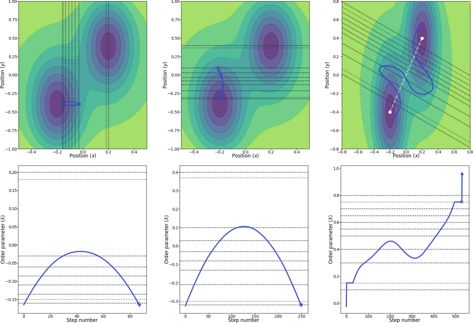
Fig. 26 Illustration of the three different order parameters with location of interfaces (dotted lines). From left to right: using the x position as the order parameter, using the y position as the order parameter and, finally, in the rightmost figure, using a combination of x and y as the order parameter. The white line in the rightmost figure show the line which we project the order parameter onto. The blue paths are valid paths for the final path ensembles and in the bottom row, the corresponding order parameters are shown for these paths. The light dotted interface lines represent the locations where we include the potential energy in the definition of the order parameters. The two marked points (cross and triangle) in the paths in the bottom row show the second last and last points in the paths, respectively. The two marked points (cross and circle) in the paths in the top row show the first and last points in the paths, respectively.

Since we include the potential energy in the order parameter definition, we will have to create customized order parameters. There is a short introduction to how the order parameters are implemented in PyRETIS in the user guide and there is also a more lengthy recipe for creating custom order parameters available.

Here, we will first consider the x (or y) order parameter and then the more involved combination.

Creating the x (or y) positional order parameter

The order parameter we are now creating will just be the position of the particle with two extra conditions:

1. If the position is below a certain value (inter_a) close to the first interface and if the potential energy is above a certain threshold value (energy_a), then the order parameter will not be allowed to come closer to the first interface.
2. If the position is closer to the last interface than a certain value (inter_b) and if the potential energy is above a certain threshold value (energy_b), then the order parameter will not be allowed to come closer to the last interface.

Thus, in addition to the position of the particle, we need to consider the 4 additional parameters inter_a, inter_b, energy_a, energy_b. The Python code for this new order parameter is given below:

Show/hide the new order parameter »

# -*- coding: utf-8 -*-
# Copyright (c) 2019, PyRETIS Development Team.
# Distributed under the LGPLv2.1+ License. See LICENSE for more info.
"""The order parameter for the hysteresis example."""
import logging
from pyretis.orderparameter.orderparameter import OrderParameter
logger = logging.getLogger(__name__)  # pylint: disable=invalid-name
logger.addHandler(logging.NullHandler())


class OrderX(OrderParameter):
    """A positional order parameter.

    Order parameter for the hysteresis example. In addition to using
    the position, we also use the energy to tell if we are in states A/B.


    Attributes
    ----------
    index : integer
        This is the index of the atom which will be used, i.e.
        system.particles.pos[index] will be used.
    inter_a : float
        An interface such that we are in state A for postions < inter_a.
    inter_b : float
        An interface such that we are in state B for postions > inter_b.
    energy_a : float
        An energy such that we are in state A for potential energy < energy_a.
    energy_b : float
        An energy such that we are in state A for potential energy < energy_b.
    dim : integer
        This is the dimension of the coordinate to use.
        0, 1 or 2 for 'x', 'y' or 'z'.
    periodic : boolean
        This determines if periodic boundaries should be applied to
        the position or not.

    """

    def __init__(self, index, inter_a, inter_b, energy_a, energy_b,
                 dim='x', periodic=False):
        """Initialise the order parameter.

        Parameters
        ----------
        index : int
            This is the index of the atom we will use the position of.
        inter_a : float
            An interface such that we are in state A for postions < inter_a.
        inter_b : float
            An interface such that we are in state B for postions > inter_b.
        energy_a : float
            An energy such that we are in state A for
            potential energy < energy_a.
        energy_b : float
            An energy such that we are in state A for
            potential energy < energy_b.
        dim : string
            This select what dimension we should consider,
            it should equal 'x', 'y' or 'z'.
        periodic : boolean, optional
            This determines if periodic boundary conditions should be
            applied to the position.

        """
        txt = 'Position of particle {} (dim: {})'.format(index, dim)
        super().__init__(description=txt)
        self.inter_a = inter_a
        self.inter_b = inter_b
        self.energy_a = energy_a
        self.energy_b = energy_b
        self.periodic = periodic
        self.index = index
        dims = {'x': 0, 'y': 1, 'z': 2}
        try:
            self.dim = dims[dim]
        except KeyError:
            msg = 'Unknown dimension {} requested'.format(dim)
            logger.critical(msg)
            raise

    def calculate(self, system):
        """Calculate the order parameter.

        Parameters
        ----------
        system : object like :py:class:`.System`
            This object is used for the actual calculation, typically
            only `system.particles.pos` and/or `system.particles.vel`
            will be used. In some cases `system.forcefield` can also be
            used to include specific energies for the order parameter.

        Returns
        -------
        out : float
            The order parameter.

        """
        particles = system.particles
        pos = particles.pos[self.index]
        lmb = pos[self.dim]
        if lmb < self.inter_a:
            if particles.vpot > self.energy_a:
                lmb = self.inter_a
        elif lmb > self.inter_b:
            if particles.vpot > self.energy_b:
                lmb = self.inter_b
        if self.periodic:
            return [system.box.pbc_coordinate_dim(lmb, self.dim)]
        return [lmb]

This new order parameter can be included in a PyRETIS simulation by adding the following order parameter section (assuming that the order parameter is stored in a file order.py):

Orderparameter
--------------
class = OrderX
module = order.py
dim = x
index = 0
periodic = False
inter_a = -0.15
inter_b = 0.18
energy_a = -9.0
energy_b = -9.0

Creating the projection-of-positions order parameter

For this order parameter, we will consider the distance from the particle to the stable A state and project the distance vector onto the line joining states A and B. In addition, as in the previously defined order parameters, we will include the energy in the definition of the states.

The Python code for this new order parameter is given below:

Show/hide the new order parameter »

# -*- coding: utf-8 -*-
# Copyright (c) 2019, PyRETIS Development Team.
# Distributed under the LGPLv2.1+ License. See LICENSE for more info.
"""This file defines the order parameter used for the WCA example."""
import logging
import numpy as np
from pyretis.orderparameter import OrderParameter
logger = logging.getLogger(__name__)  # pylint: disable=invalid-name
logger.addHandler(logging.NullHandler())


class OrderXY(OrderParameter):
    """OrderXY(OrderParameter).

    This class defines a 2D order parameter such that x + y = constant.

    Attributes
    ----------
    index : integer
        This selects the particle to use for the order parameter.
    inter_a : float
        An interface such that we are in state A for postions < inter_a.
    inter_b : float
        An interface such that we are in state B for postions > inter_b.
    energy_a : float
        An energy such that we are in state A for potential energy < energy_a.
    energy_b : float
        An energy such that we are in state A for potential energy < energy_b.

    """

    def __init__(self, index, inter_a, inter_b, energy_a, energy_b):
        """Set up the order parameter.

        Parameters
        ----------
        index : tuple of ints
            This is the indices of the atom we will use the position of.
        inter_a : float
            An interface such that we are in state A for postions < inter_a.
        inter_b : float
            An interface such that we are in state B for postions > inter_b.
        energy_a : float
            An energy such that we are in state A for
            potential energy < energy_a.
        energy_b : float
            An energy such that we are in state A for
            potential energy < energy_b.

        """
        super().__init__(description='2D->1D projection')
        self.index = index
        x_1 = 0.2
        y_1 = 0.4
        x_0 = -0.2
        y_0 = -0.4
        self.x_0 = x_0
        self.y_0 = y_0
        self.origin = np.array([x_0, y_0])
        self.vec = np.array([x_1 - x_0, y_1 - y_0])
        self.vec /= np.sqrt(np.dot(self.vec, self.vec))
        self.inter_a = inter_a
        self.inter_b = inter_b
        self.energy_a = energy_a
        self.energy_b = energy_b

    def calculate(self, system):
        """Calculate the order parameter.

        Here, the order parameter is just the distance between two
        particles.

        Parameters
        ----------
        system : object like :py:class:`.System`
            This object is used for the actual calculation, typically
            only `system.particles.pos` and/or `system.particles.vel`
            will be used. In some cases `system.forcefield` can also be
            used to include specific energies for the order parameter.

        Returns
        -------
        out : float
            The order parameter.

        """
        pos = system.particles.pos[self.index]
        vec = np.array([pos[0] - self.x_0, pos[1] - self.y_0])
        proj = np.dot(vec, self.vec)
        if proj < self.inter_a:
            if system.particles.vpot > self.energy_a:
                proj = self.inter_a
        elif proj > self.inter_b:
            if system.particles.vpot > self.energy_b:
                proj = self.inter_b
        return [proj]

Note that this order parameter is less general than the previous ones, for instance, we make explicit use of the location of the two minimums. If you are feeling adventurous, please try to add these locations as parameters for the order parameter.

This new order parameter can be included in a PyRETIS simulation by adding the following order parameter section (assuming that the order parameter is stored in a file order.py):

Orderparameter
--------------
class = OrderXY
module = orderp.py
index = 0
inter_a = 0.15
inter_b = 0.75
energy_a = -9.0
energy_b = -9.0

Running the RETIS simulation with PyRETIS

We have now defined the potential and the order parameters we are going to use and we are ready to run the RETIS simulations.

Running the RETIS simulation using x as the order parameter

In order to run the RETIS simulation, the following steps are suggested:

1. Create a new folder, for instance 2D-hysteresis.

2. Place the order parameter script in this folder and name it order.py.

3. Download the initial configuration initial.xyz and place it in the same directory.

4. Create a new sub-directory, retis-x.

5. Add the following input script retis-x.rst to the retis-x folder.

6. Run the simulation using (in the retis-x folder):

   pyretisrun -i retis-x.rst -p
   

Some examples from the analysis can be found below:

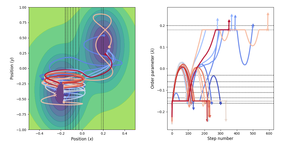
Fig. 27 Example of paths harvested for the RETIS simulation. All paths shown are accepted paths for the last path ensemble.

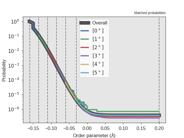
Fig. 28 The crossing probability after 1 000 000 RETIS cycles. The numerical value 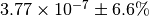is . The initial flux is .

Running the RETIS simulation using y as the order parameter

In order to run the RETIS simulation, the following steps are suggested:

1. Create a new folder, for instance 2D-hysteresis.

2. Place the order parameter script in this folder and name it order.py.

3. Download the initial configuration initial.xyz and place it in the same directory.

4. Create a new sub-directory, retis-y.

5. Add the following input script retis-y.rst to the retis-y folder.

6. Run the simulation using (in the retis-y folder):

   pyretisrun -i retis-y.rst -p
   

Some examples from the analysis can be found below:

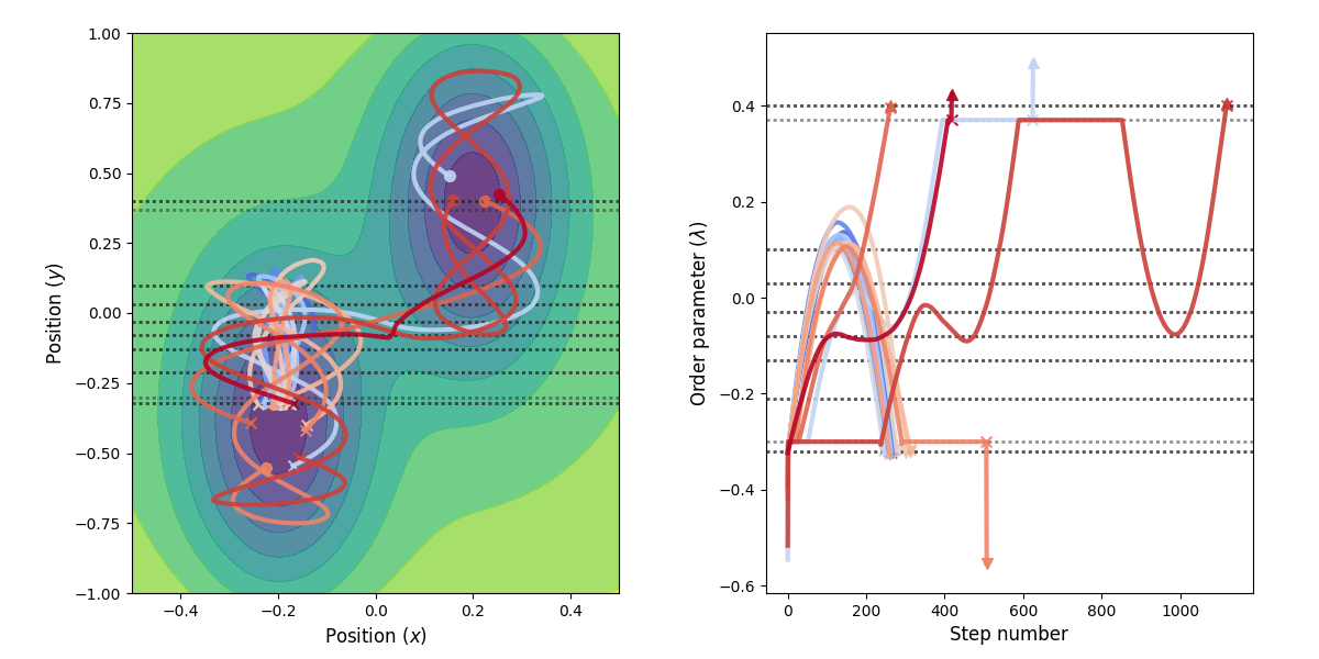
Fig. 29 Example of paths harvested for the RETIS simulation. All paths shown are accepted paths for the last path ensemble.

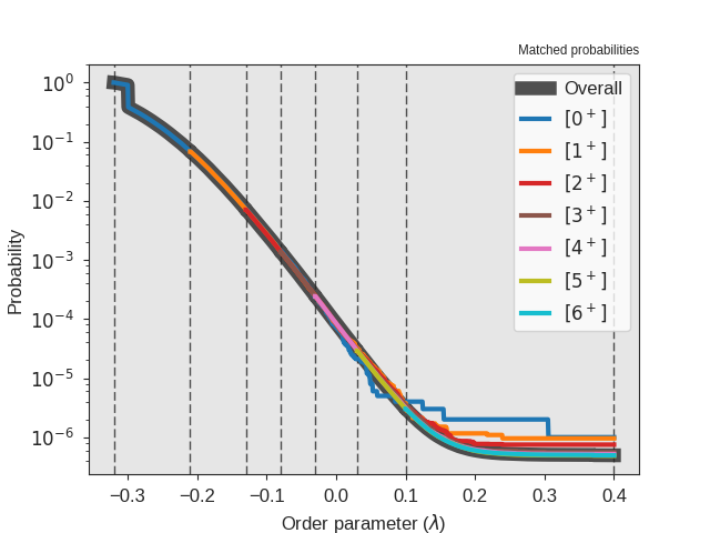
Fig. 30 The crossing probability after 1 000 000 RETIS cycles. The numerical value 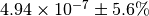is . The initial flux is .

Running the RETIS simulation using the projection-of-position as the order parameter

In order to run the RETIS simulation, the following steps are suggested:

1. Create a new folder, for instance 2D-hysteresis.

2. Create a new sub-directory, retis-xy and move into this directory.

3. Place the order parameter script in this folder and name it order.py.

4. Download the initial configuration initial2.xyz and place it in the same directory and rename it to initial.xyz.

5. Add the following input script retis-xy.rst to the retis-xy folder.

6. Run the simulation using (still in the retis-xy folder):

   pyretisrun -i retis-xy.rst -p
   

Some examples from the analysis can be found below:

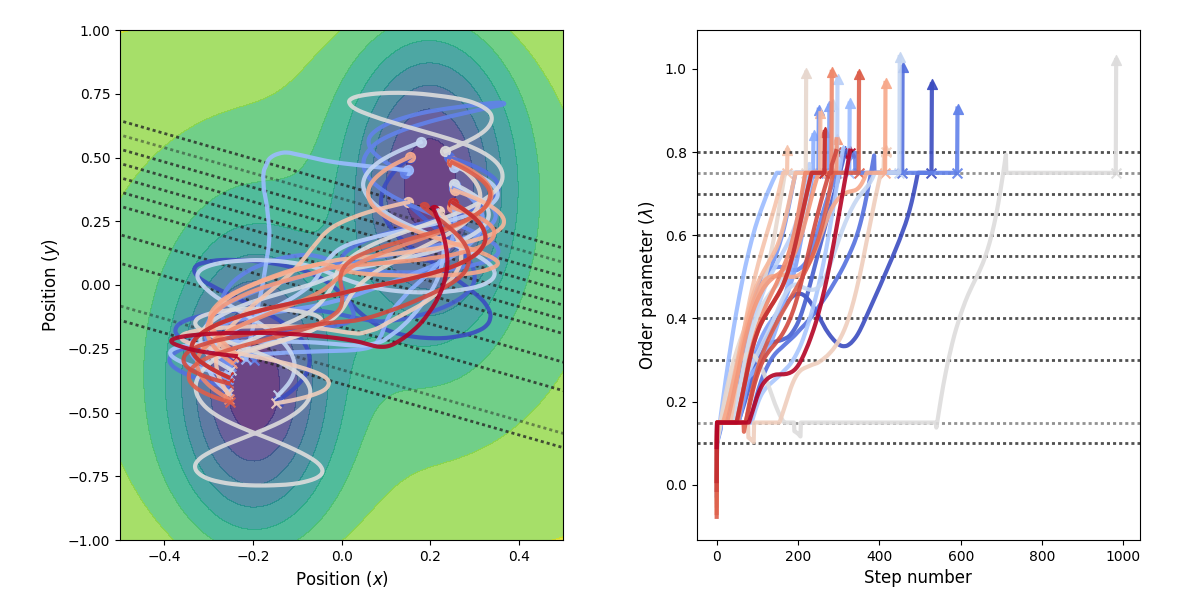
Fig. 31 Example of paths harvested for the RETIS simulation. All paths shown are accepted paths for the last path ensemble.

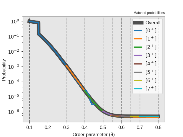
Fig. 32 The crossing probability after 1 000 000 RETIS cycles. The numerical value 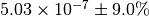is . The initial flux is .

Comparing results from the analysis

By using the three different order parameters, we obtain different estimates for the rate constant as summarized in the table below.

Table 50 Comparison of the rate constant for the 2D potential

Order parameter	Rate constant / 1e-7
	Lower bound	Upper bound
x	7.3	8.3
y	7.7	8.6
xy	7.3	8.3