Molecular dynamics examples
In this example, we will perform a MD simulation of a Lennard-Jones fluid. The purpose of this example is to illustrate two different ways we can use PyRETIS:
- Running the simulation using an input file and the PyRETIS executable
- Running the simulation by making explicit use of the PyRETIS library
The simulation we set up is rather ordinary and we will start from a regular lattice and simulate the melting at a specified temperature as illustrated in the figure below.
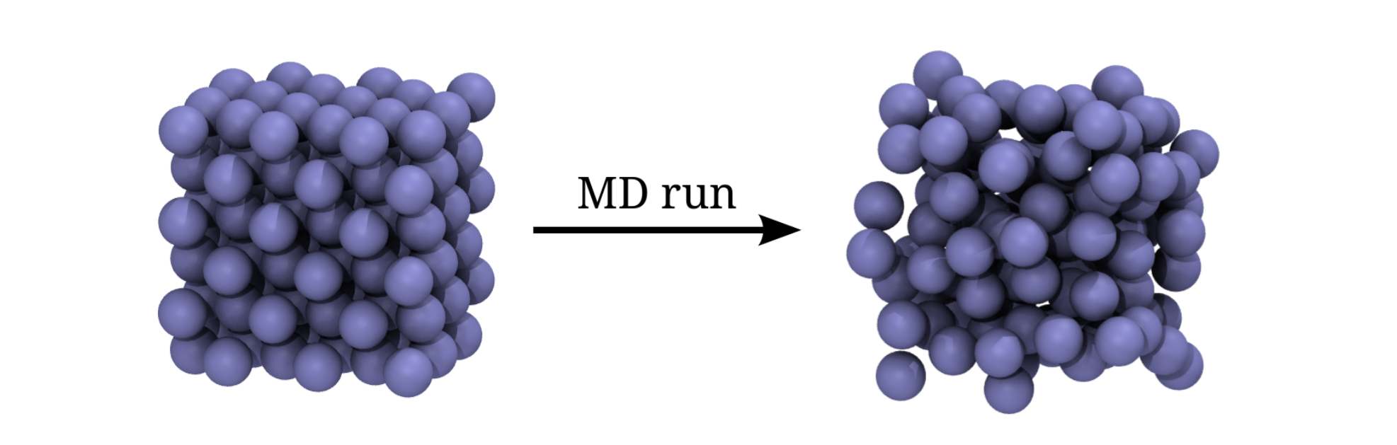
Fig. 15 The initial (left) and the final structure (right) of the Lennard-Jones simulation. The initial structure is a FCC lattice, while the final structure is less ordered.
Table of Contents
Molecular dynamics using an input file
We can execute PyRETIS by creating an input file and using
the PyRETIS application.
In order to run this example, merge the code-snippets given below
into one file, say md.rst, which then can be executed by:
pyretisrun -i md.rst
In the first part of the input file, we will specify the type of simulation to run and the number of steps to perform by defining the simulation section:
Molecular dynamics example settings
===================================

Simulation settings
-------------------
task = md-nve
steps = 1000
In order to produce some actual dynamics, we will have to integrate the equations of motion. The engine to use for this is selected using the engine section:
Engine settings
---------------
class = velocityverlet
timestep = 0.002
and we define the system we are studying using the system section and the particles section: and the particles:
System settings
---------------
temperature = 2.0
units = lj

Particles
---------
position = {'generate': 'fcc',
            'repeat': [3, 3, 3],
            'density': 0.9}

velocity = {'generate': 'maxwell',
            'temperature': 2.0,
            'momentum': True,
            'seed': 0}

mass = {'Ar': 1.0}
name = ['Ar']
type = [0]
We also need to specify a force field, which is done by specifying the forcefield section and one or more potential sections. In this case, the force field is set up using a single type of potential function:
Forcefield settings
-------------------
description = Lennard Jones test

Potential
---------
class = PairLennardJonesCutnp
shift = True
parameter 0 = {'sigma': 1.0, 'epsilon': 1.0, 'rcut': 2.5}
and we modify the output created by specifying the output section:
Output
------
backup = overwrite
energy-file = 1
order-file = 10
cross-file = 1
trajectory-file = 10
What we are essentially modifying here is
the frequency of the output, and we are also telling PyRETIS
not to back-up, but to overwrite old output files that might
be present in the same directory (this is controlled
by the backup = False keyword setting).
After running this example, the following files should have been created:
energy.txt- This file contains energies and temperature as a function of time/step in the MD simulation:
thermo.txt- This file contains the same energies as
energy.txtand in addition the pressure.
traj.xyz- This file contains the trajectory and can be visualised using for instance VMD.
pyretis.log- This file contains output messages from the PyRETIS application.
out.rst- This file contains the input settings you provided as PyRETIS read them. This can be used to check the correctness of the input file.
Plotting the pressure from thermo.txt should then give
a figure similar to:
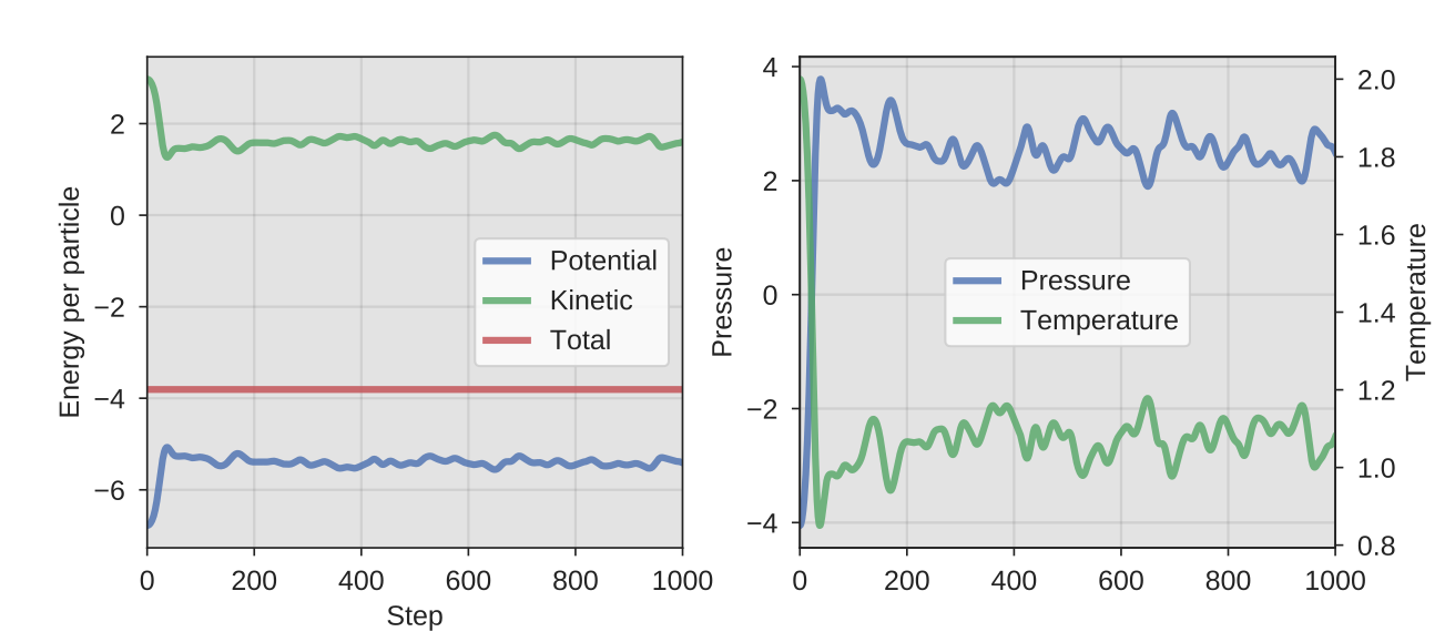
Fig. 16 A representative output from the MD NVE simulation: The eneriges, pressure and the temperature as a function of the simulation step.
Molecular dynamics using the PyRETIS library
In this part of the example, we will make explicit use
of the PyRETIS library
If you want
to try this example, you will have to copy the code-snippets
given below into a Python script, say md.py, and run it as
python md.py
This example is best understood if you have read about the PyRETIS API.
We begin the example by importing from the PyRETIS library:
import sys
import numpy as np
from pyretis.core import create_box, Particles, System
from pyretis.simulation import SimulationNVE
from pyretis.engines import VelocityVerlet
from pyretis.tools import generate_lattice
from pyretis.forcefield import ForceField
from pyretis.forcefield.potentials import PairLennardJonesCutnp
We also import Numpy and matplotlib here in order to do some plotting. If you want a more fancy plot and have a recent version of matplotlib installed you can try to use one of the many styles, e.g.:
# the plot nicer by loading a style, e.g.:
Next, we create the initial positions and use this to set up a simulation box:
def set_up_system():
    """Set up a system using the PyRETIS library."""
We can use the lattice we generated to populate a system with particles. The system contains information about the box, the particles and the temperature:
    xyz, size = generate_lattice('fcc', [3, 3, 3], density=0.9)
    size = np.array(size)
    box = create_box(low=size[:, 0], high=size[:, 1])
    print(box)

    print('Creating system:')
    system = System(units='lj', box=box, temperature=2.0)
    system.particles = Particles(dim=3)
    for pos in xyz:
In the last lines in the above code, we generated initial velocities,
from a Maxwellian distribution such that the total
momentum of the system is zero (requested by setting the
key 'momentum' to True in the dictionary).
Now, we just have to set-up a force field:
                            force=np.zeros_like(pos),
                            mass=1.0, name='Ar', ptype=0)

    gen_settings = {'distribution': 'maxwell', 'momentum': True}
    system.generate_velocities(**gen_settings)
    print(system.particles)
select an engine and a simulation to run:
    potentials = [PairLennardJonesCutnp(dim=3, shift=True, mixing='geometric')]
    parameters = [{0: {'sigma': 1, 'epsilon': 1, 'rcut': 2.5}}]
    ffield = ForceField('Lennard Jones force field',
Now, we are ready to run the simulation and plot the energies as a function of the simulation step:
    system.forcefield = ffield
    print(system.forcefield)
    return system


def set_up_simulation(system):
    """Set up the simulation."""
    print('Creating simulation:')
    engine = VelocityVerlet(0.002)
    simulation = SimulationNVE(system, engine, steps=200)
    return simulation


def run_simulation(simulation):
    """Run the simulation and collect some outputs."""
    ekin = []
    vpot = []
    etot = []
    step = []
    for result in simulation.run():
        if result['cycle']['step'] % 10 == 0:
            print('Step:', result['cycle']['step'])
        step.append(result['cycle']['step'])
This should result in a plot similar to:
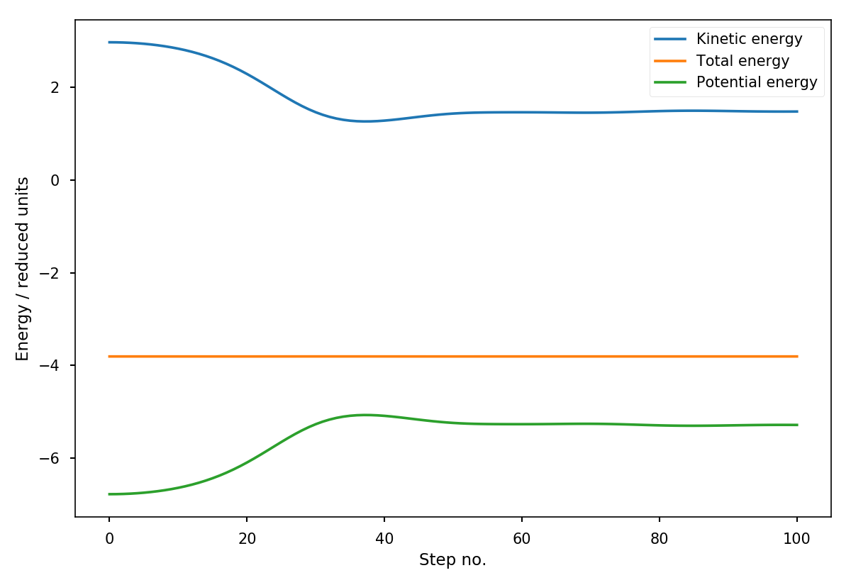
Fig. 17 Energies as a function of the time in the MD simulation.