Particle Swarm Optimization¶

In this example, we will perform a task that PyRETIS is NOT intended to do. We will optimize a function using a method called particle swarm optimization and the purpose of this example is to illustrate how the PyRETIS library can be used to set up special simulations.

The function we will optimize is the Ackley function which is relatively complex with many local minima as illustrated in the figure below. We will set up our optimization by first creating a new potential and a new engine to do the job for us.

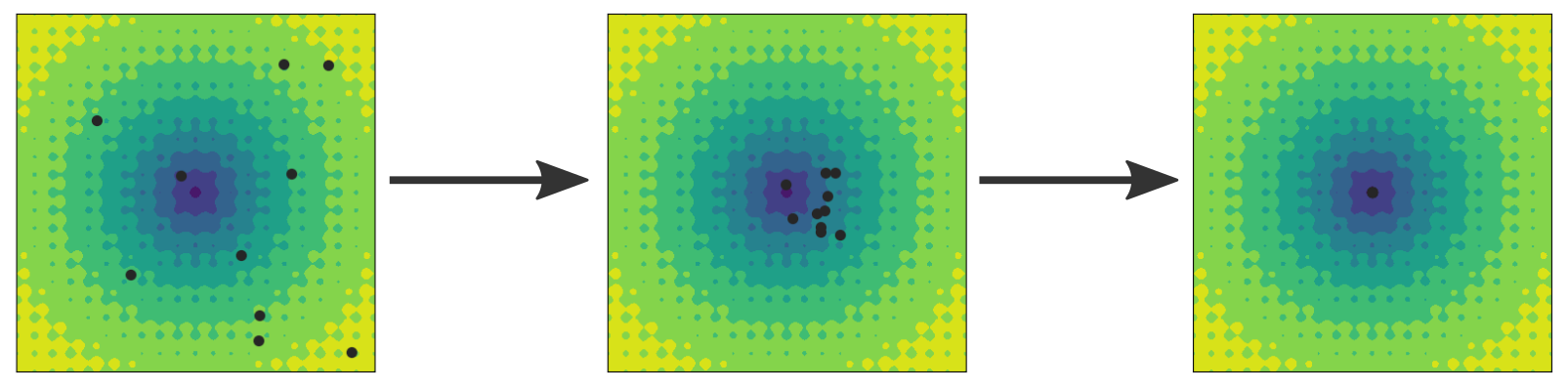
Illustration of particle swarm optimization

Fig. 37 Illustration of the particle swarm optimization method. The particles (black circles) start in a random initial configuration as shown in the left image and search for the global minimum. All particles keep a record of the smallest value they have seen so far and they communicate this estimate to the other particles. Thus, the current best estimate based on all the particles is known, and the particles are drawn towards this position, but also towards their own best estimate. In the middle image, the positions have been updated and the particles have moved. After some more steps, the particles converge towards the global minimum at (0, 0). However, convergence is not guaranteed.¶

Table of Contents

Creating the Ackley function as a PotentialFunction
Creating a custom engine for particle swarm optimization
Putting it all together and running the optimization
Adding plotting and animation

Creating the Ackley function as a PotentialFunction ¶

Here, we will create the function we will optimize as a PotentialFunction. This can be done by creating a new file ackley.py and adding the following code:

import numpy as np
from matplotlib import pyplot as plt
from mpl_toolkits.mplot3d import Axes3D  # pylint: disable=unused-import
from pyretis.forcefield import PotentialFunction


TWO_PI = np.pi * 2.0
EXP = np.exp(1)


@np.vectorize
def ackley_potential(x, y):  # pylint: disable=invalid-name
    """Evaluate the Ackley function."""
    return (-20.0 * np.exp(-0.2*np.sqrt(0.5*(x**2 + y**2))) -
            np.exp(0.5 * (np.cos(TWO_PI * x) + np.cos(TWO_PI * y))) +
            EXP + 20)


class Ackley(PotentialFunction):
    """A implementation of the Ackley function.

    Note that the usage of this potential function differs from
    the usual usage for force fields.

    """

    def __init__(self):
        """Set up the function."""
        super().__init__(dim=2, desc='The Ackley function')

    def potential(self, system):
        """Evaluate the potential, note that we return all values."""
        xpos = system.particles.pos[:, 0]
        ypos = system.particles.pos[:, 1]
        pot = ackley_potential(xpos, ypos)
        return pot

If you add:

def main():
    """Plot the Ackley function."""
    xgrid, ygrid = np.meshgrid(np.linspace(-5, 5, 100),
                               np.linspace(-5, 5, 100))
    zgrid = ackley_potential(xgrid, ygrid)

    fig = plt.figure()
    ax1 = fig.add_subplot(211)
    ax2 = fig.add_subplot(212, projection='3d')
    ax1.contourf(xgrid, ygrid, zgrid)
    ax2.plot_surface(xgrid, ygrid, zgrid, cmap=plt.get_cmap('viridis'))
    plt.show()


if __name__ == '__main__':
    main()

you can also plot the potential by running:

python ackley.py

Creating a custom engine for particle swarm optimization ¶

Here, we will create a new engine for performing the “dynamics” in the particle swarm optimization. The equations of motion are

For the velocity $v_i$ of particle i:

$v_i(t + 1) = \omega v_i(t) + c_1 r_1 (x_i^\ast - x_i(t)) + c_2 r_2 (x^\dagger - x_i(t))$

where $\omega$ is the co-called inertia weight (a parameter), $c_1$ and $c_2$ are acceleration coefficients (parameters), $r_1$ and $r_2$ are random numbers drawn from a uniform distribution between 0 and 1, $x_i^\ast$ is particle i’s best estimate of the minimum of the potential and $x^\dagger$ is the global best estimate.
For the position $x_i$ of particle i:

$x_i(t + 1) = x_i(t) + v_i(t)$

In both equations, $t$ is the current step and $t+1$ is the next step. Before updating the positions, the potential energies for the individual particles are obtained and $x_i^\ast$ and $x^\dagger$ are updated.

These equations are similar to the equations used by the MD integrators in PyRETIS, and the engine can be implemented as a sub-class of the MDEngine class. Create a new file name psoengine.py and add the following code:

# -*- coding: utf-8 -*-
# Copyright (c) 2019, PyRETIS Development Team.
# Distributed under the LGPLv2.1+ License. See LICENSE for more info.
"""A custom engine for particle swarm optimization."""
import numpy as np
from pyretis.engines import MDEngine


class PSOEngine(MDEngine):
    """Perform particle swarm optimization."""

    def __init__(self, inertia, accp, accg):
        """Set up the engine.

        Parameters
        ----------
        intertia : float
            The intertia factor in the velocity equation
            of motion.
        accp : float
            The acceleration for the previous best term. "The congnitive term".
        accg : float
            The acceleration for the global best term. "The social term".

        """
        super().__init__(1, 'Particle Swarm Optimization')
        self.inertia = inertia
        self.accp = accp
        self.accg = accg
        self.pbest = None
        self.pbest_pot = None
        self.gbest = None
        self.gbest_pot = None

    def integration_step(self, system):
        """Perform one step for the PSO algorithm."""
        particles = system.particles
        if self.pbest is None:
            self.pbest = np.copy(particles.pos)
            self.pbest_pot = system.potential()
        if self.gbest is None:
            pot = system.potential()
            idx = np.argmin(pot)
            self.gbest = particles.pos[idx]
            self.gbest_pot = pot[idx]

        rnd1 = np.random.uniform()
        rnd2 = np.random.uniform()

        particles.vel = (self.inertia * particles.vel +
                         rnd1 * self.accp * (self.pbest - particles.pos) +
                         rnd2 * self.accg * (self.gbest - particles.pos))
        particles.pos += particles.vel
        particles.pos = system.box.pbc_wrap(particles.pos)

        pot = system.potential()

        # Update global?
        idx = np.argmin(pot)
        if pot[idx] < self.gbest_pot:
            self.gbest_pot = pot[idx]
            self.gbest = particles.pos[idx]
        # Update for individuals:
        idx = np.where(pot < self.pbest_pot)[0]
        self.pbest[idx] = np.copy(particles.pos[idx])
        self.pbest_pot[idx] = pot[idx]
        return self.gbest_pot, self.gbest

Putting it all together and running the optimization ¶

We will now create a simulation for performing the optimization. First, we need to import the new potential function and the new engine we have created:

import numpy as np
from pyretis.core import create_box, Particles, System
from pyretis.simulation import Simulation
from pyretis.forcefield import ForceField
from psoengine import PSOEngine
from ackley import Ackley, ackley_potential

We next use this to define a method for setting everything up for us:

NPART = 10
STEPS = 1000
MINX, MAXX = -10, 10
TXT = 'Step: {:5d}: Best: (x, y) = ({:10.3e}, {:10.3e}), pot = {:10.3e}'


def set_up():
    """Just create system and simulation."""
    box = create_box(low=[MINX, MINX], high=[MAXX, MAXX],
                     periodic=[True, True])
    print('Created a box:')
    print(box)

    print('Creating system with {} particles'.format(NPART))
    system = System(units='reduced', box=box)
    system.particles = Particles(dim=2)
    for _ in range(NPART):
        pos = np.random.uniform(low=MINX, high=MAXX, size=(1, 2))
        system.add_particle(pos)

    ffield = ForceField('Single Ackley function',
                        potential=[Ackley()])
    system.forcefield = ffield
    print('Force field is:\n{}'.format(system.forcefield))

    print('Creating simulation:')
    engine = PSOEngine(0.7, 1.5, 1.5)
    simulation = Simulation(steps=STEPS)
    task_integrate = {'func': engine.integration_step,
                      'args': [system],
                      'result': 'gbest', 'first': True}
    simulation.add_task(task_integrate)
    return simulation, system

Finally, we can make a method to execute the optimization:

def main():
    """Just run the optimization, no plotting."""
    simulation, _ = set_up()
    for result in simulation.run():
        step = result['cycle']['step']
        best = result['gbest']
        if step % 10 == 0:
            print(TXT.format(step, best[1][0], best[1][1], best[0]))

Which is used as follows:

if __name__ == '__main__':
    main()

Execute the script a couple of time (save the code above in a new file, say pso_run.py) and execute it using:

python pso_run.py

Adding plotting and animation ¶

If you wish, you can also animate the results/optimization process. First modify the imports as follows:

import numpy as np
from pyretis.core import create_box, Particles, System
from pyretis.simulation import Simulation
from pyretis.forcefield import ForceField
from psoengine import PSOEngine
from ackley import Ackley, ackley_potential
from matplotlib import pyplot as plt
from matplotlib import animation, cm

And add the following methods:

def evaluate_potential_grid():
    """Evaluate the Ackley potential on a grid."""
    X, Y = np.meshgrid(np.linspace(MINX, MAXX, 100),
                       np.linspace(MINX, MAXX, 100))
    Z = ackley_potential(X, Y)
    return X, Y, Z


def update_animation(frame, system, simulation, scatter):
    """Update animation."""
    patches = []
    if not simulation.is_finished() and frame > 0:
        results = simulation.step()
        best = results['gbest']
        if frame % 10 == 0:
            print(TXT.format(frame, best[1][0], best[1][1], best[0]))
    scatter.set_offsets(system.particles.pos)
    patches.append(scatter)
    return patches


def main_animation():
    """Run the simulation and update for animation."""
    simulation, system = set_up()
    fig = plt.figure()
    ax1 = fig.add_subplot(111, aspect='equal')
    ax1.set_xlim((MINX, MAXX))
    ax1.set_ylim((MINX, MAXX))
    ax1.axes.get_xaxis().set_visible(False)
    ax1.axes.get_yaxis().set_visible(False)
    X, Y, pot = evaluate_potential_grid()
    ax1.contourf(X, Y, pot, cmap=cm.viridis, zorder=1)
    scatter = ax1.scatter(system.particles.pos[:, 0],
                          system.particles.pos[:, 1], marker='o', s=50,
                          edgecolor='#262626', facecolor='white')

    def init():
        """Just return what to re-draw."""
        return [scatter]
    # This will run the animation/simulation:
    anim = animation.FuncAnimation(fig, update_animation,
                                   frames=STEPS+1,
                                   fargs=[system, simulation, scatter],
                                   repeat=False, interval=30, blit=True,
                                   init_func=init)
    plt.show()
    return anim


if __name__ == '__main__':
    main_animation()

Particle Swarm Optimization¶

Creating the Ackley function as a PotentialFunction¶

Creating a custom engine for particle swarm optimization¶

Putting it all together and running the optimization¶

Adding plotting and animation¶

Creating the Ackley function as a PotentialFunction ¶

Creating a custom engine for particle swarm optimization ¶

Putting it all together and running the optimization ¶

Adding plotting and animation ¶