Subtrajectory moves in a 1D potential
This example shows how to use the subtrajectory monte carlo moves Stone Skipping (SS), Web Throwing (WT) [1] and Wire Fencing (WF) [2] in (Replica Exchange) Transition Interface Sampling simulations for sampling trajectories of a particle in a 1D well. The three moves are sketched out below:
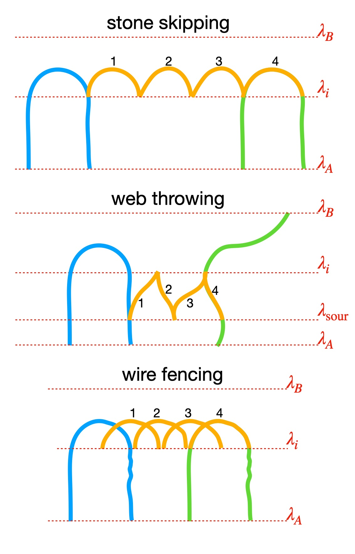
Fig. 30 Cartoon representation of the three subtrajectory moves: stone skipping, web throwing and web throwing. The old path is shown in blue. Four subtrajectories are shown in orange. The final new path consists of the fourth subtrajectory and its extensions in green.
Further details on the 1D potential, how to create the PyRETIS input file and calculating reaction rates using TIS/RETIS are explained by the previous 1D potential TIS example and RETIS example.
Verification status: passing – see Tutorial map.
Tutorial quick start
Best starting point:
examples/tutorials/path_sampling/internal/1D-double-well/submoves/.Edit first: the
shooting_moves,interface_sour,interface_cap, andn_jumpssettings in theTISsection.Run:
pyretis run -i retis.toml -pfrom the tutorial folder.Analyse:
pyretis analyse -i retis.tomlafter the run.Expected output: standard RETIS ensemble folders plus move labels for stone skipping, web throwing, and wire fencing in
pathensemble.txt.Related check:
examples/tests/test-internal/retis-ss-wt-wf/; see Example test status.
Defining the shooting move
To define the specific shooting moves performed in each of the
ensembles in i.e. a RETIS simulation, the number of ensembles
needs to be known. This information can be obtained from reading
the interfaces variable in the
simulation section of the input file:
[simulation]
task = "retis"
steps = 200
interfaces = [
    -0.99,
    -0.8,
    -0.7,
    -0.6,
    -0.5,
    -0.4,
    -0.3,
    1.0,
]
Here we have one \([0^{-}]\) ensemble and seven \([i^{+}]\) ensembles for a total of 8 ensembles. Then we can define the specific shooting moves to be performed in each ensemble in the tis section:
[tis]
freq = 0.0
maxlength = 50000
allowmaxlength = false
zero_momentum = false
rescale_energy = false
sigma_v = -1
seed = 0
shooting_moves = [
    "sh",
    "sh",
    "ss",
    "ss",
    "wt",
    "wt",
    "wf",
    "wf",
]
interface_sour = -0.8
interface_cap = 0.1
n_jumps = 6
high_accept = true
The shooting_moves variable defines the list of shooting moves
to be used for all the ensembles. Here we see that \([0^{-}]\) and
\([0^{+}]\) performs the shooting move while the other
ensembles performs the SS, WT and WF moves. The interface_sour
sets the SOUR interface for the WT, while
if defined, the interface_cap variable sets the upper value
limit of subtrajectories generated by the WF move. The variable
n_jumps defines the number of subtrajectories to be generated
per move and the bool high_accept determines whether the
high acceptance protocol should be used or not.
See Move types for the full list of move type
codes and Path status codes for all acceptance and
rejection status codes.
Running the RETIS simulation
Running a RETIS simulation with subtrajectory moves works the same way
as running without subtrajectory moves. Below is the complete
retis.toml input file.
Show/hide the full input file »
potential = [
    { class = "DoubleWell", a = 1.0, b = 2.0, c = 0.0 },
]

[simulation]
task = "retis"
steps = 200
interfaces = [
    -0.99,
    -0.8,
    -0.7,
    -0.6,
    -0.5,
    -0.4,
    -0.3,
    1.0,
]

[system]
units = "reduced"
dimensions = 1
temperature = 0.07

[engine]
class = "Langevin"
timestep = 0.025
gamma = 0.3
high_friction = false
seed = 0

[box]
periodic = [
    false,
]

[particles]
name = [
    "Ar",
]
ptype = [
    0,
]

[particles.position]
input_file = "initial.xyz"

[particles.mass]
Ar = 1.0

[forcefield]
description = "1D double well"

[orderparameter]
class = "Position"
dim = "x"
index = 0
periodic = false

[output]
archive_every = 50
backup = "overwrite"
order-file = -1
trajectory-file = -1
energy-file = -1

[tis]
freq = 0.0
maxlength = 50000
allowmaxlength = false
zero_momentum = false
rescale_energy = false
sigma_v = -1
seed = 0
shooting_moves = [
    "sh",
    "sh",
    "ss",
    "ss",
    "wt",
    "wt",
    "wf",
    "wf",
]
interface_sour = -0.8
interface_cap = 0.1
n_jumps = 6
high_accept = true

[initial-path]
method = "kick"
kick-from = "initial"

[retis]
swapfreq = 0.5
nullmoves = true
swapsimul = true
The initial configuration
initial.xyz
is included in the tutorial folder. The simulation can then be
executed using:
pyretis run -i retis.toml -p
The -p option will display a progress bar for your simulation.
Tested by
The subtrajectory move settings are represented by
examples/tutorials/path_sampling/internal/1D-double-well/submoves/ and
checked by examples/tests/test-internal/retis-ss-wt-wf/. Use
the fixture as the short regression check and this page as the
user-facing guide to choosing and interpreting the move settings.