Umbrella Sampling
This example will simply calculate the free energy profile in a given, known, potential using umbrella sampling. The results we will obtain are shown in the figure below: the potential energy \(V(x)\) and the probability density.
Verification status: smoke – see Tutorial map.
Tutorial quick start
Best starting point:
examples/tutorials/umbrella_sampling/.Edit first:
umbrella_sampling_mc.pyfor umbrella windows, force-field parameters, and the number of Monte Carlo cycles.Run:
python umbrella_sampling_mc.py.Expected output: terminal progress for each umbrella window and a plot of the reconstructed probability/free-energy profile.
Short check:
examples/run-tutorials.shstarts this script with a timeout.Related checks: no dedicated heavy-test fixture yet; see Example test status.
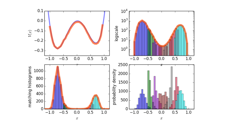
Fig. 31 Sample results for the potential energy and the probability density.
We begin by importing the PyRETIS library and numpy and matplotlib which we will use for some additional numerical methods and for plotting.
import numpy as np
from matplotlib import pyplot as plt
from pyretis.core import System, RandomGenerator, Particles
from pyretis.simulation.mc_simulation import UmbrellaWindowSimulation
from pyretis.forcefield import ForceField
from pyretis.forcefield.potentials import DoubleWell, RectangularWell
from pyretis.analysis import histogram, match_all_histograms
First, we set up the system by defining the units we will use and adding a particle (labeled as ‘X’) at a specified position.
mysystem = System(temperature=500, units='eV/K')
mysystem.particles = Particles(dim=1)
mysystem.add_particle(name='X', pos=np.array([-0.7]))
Next we define the force field in terms of potential functions. Here, we create the unbiased potential - a double well potential - and a biased version of the potential where a rectangular well is used. Finally, the biased force field is attached to the system.
potential_dw = DoubleWell(a=1, b=1, c=0.02)
potential_rw = RectangularWell()
forcefield = ForceField(desc='Double well', potential=[potential_dw])
forcefield_bias = ForceField(desc='Double well with rectangular bias',
                             potential=[potential_dw, potential_rw])
mysystem.forcefield = forcefield_bias
In order to run the actual simulation, we need to specify some additional settings, like where the umbrella windows should be placed and how many cycles we need to perform:
umbrellas = [[-1.0, -0.4], [-0.5, -0.2], [-0.3, 0.0],
             [-0.1, 0.2], [0.1, 0.4], [0.3, 0.6], [0.5, 1.0]]
n_umb = len(umbrellas)
MINCYCLES = 1e4  # Number of MC steps to perform.
MAXDX = 0.1  # Maximum allowed displacement in the MC step(s).
and we create a random number generator for use in the umbrella simulation:
RANDSEED = 1  # Seed for the random number generator:
RGEN = RandomGenerator(seed=RANDSEED)
We are now ready to run the simulation. We will do this by looping over the umbrella windows we defined,
trajectory, energy = [], []  # For storing trajectories & energies.
for i, umbrella in enumerate(umbrellas):
    print('Running umbrealla no: {} of {}. Location: {}'.format(i + 1, n_umb,
                                                                umbrella))
    # Move rectangular potential to correct place:
    params = {'left': umbrella[0], 'right': umbrella[1]}
    mysystem.forcefield.update_potential_parameters(potential_rw, params)
    mysystem.potential()  # Re-calculate potential energy.
    over = umbrellas[min(i + 1, n_umb - 1)][0]  # Position we must cross.
    simulation = UmbrellaWindowSimulation(
        ensemble={
            'system': mysystem,
            'rgen': RGEN
        },
        settings={
            'simulation': {
                'task': 'umbrella',
                'umbrella': umbrella,
                'overlap': over,
                'maxdx': MAXDX
            }
        },
        controls={'steps': MINCYCLES}
    )
    # Also create empy list for storing some data:
    traj, ener = [], []
    for result in simulation.run():
        for pos in mysystem.pos:
            traj.append(pos)
            ener.append(mysystem.particles.vpot)
    trajectory.append(np.array(traj))
    energy.append(np.array(ener))
    print('Done. Cycles: {}'.format(simulation.cycle['stepno']))
The simulation is now done, and we can do the analysis and plot the results. For the analysis we match the histograms:
# We can now post-process the simulation output:
BINS = 100
LIM = (-1.1, 1.1)
histograms = [histogram(traj, bins=BINS, limits=LIM) for traj in trajectory]
# Extract the bins (the midpoints) and the bin-width:
bin_x = histograms[0][-1]
dbin = bin_x[1] - bin_x[0]
# We are going to match these histograms:
print('Matching histograms...')
histograms_s, _, hist_avg = match_all_histograms(histograms, umbrellas)
And we finally plot the results:
print('Plotting matched histograms')
fig = plt.figure()
axs = fig.add_subplot(111)
axs.set_yscale('log')
axs.set_xlabel('Position ($x$)', fontsize='large')
axs.set_ylabel('Matched histograms', fontsize='large')
colors = ['blue', 'green', 'darkviolet', 'brown', 'gray', 'crimson', 'cyan']
for i, histo in enumerate(histograms_s):
    axs.bar(bin_x - 0.5 * dbin, histo, dbin, color=colors[i],
            alpha=0.6, log=True)
axs.plot(bin_x, hist_avg, lw=7, color='orangered', alpha=0.6,
         label='Average after matching')
axs.legend()
plt.xlim((-1.1, 1.1))

print('Plotting the free energy')
fig2 = plt.figure()
ax2 = fig2.add_subplot(111)
XPOT = np.linspace(-2, 2, 1000)
free = -np.log(hist_avg) / mysystem.temperature['beta']  # The free energy.
# Set up unbiased potential for plotting:
VPOT = []
for xi in XPOT:
    mysystem.pos = xi
    VPOT.append(forcefield.evaluate_potential(mysystem))
VPOT = np.array(VPOT)
free += (VPOT.min() - free.min())
ax2.plot(XPOT, VPOT, 'blue', lw=3, label='Unbiased potential', alpha=0.5)
ax2.plot(bin_x, free, lw=7, alpha=0.5, color='green', label='Free energy')
ax2.set_xlabel('Position ($x$)', fontsize='large')
ax2.set_ylabel('Potential energy ($V(x)$) / eV', fontsize='large')
ax2.legend()
plt.xlim((-1.1, 1.1))
plt.ylim((-0.3, 0.05))
plt.show()
Tested by
This tutorial is covered by the tutorial smoke runner, which verifies
that the script starts and performs Monte Carlo cycles with the current
PyRETIS installation. Add a shortened fixture under
examples/tests/ before treating umbrella sampling as part of the
heavy regression suite.