Simulation outputs¶

A PyRETIS run leaves behind a directory of plain-text files, and pyretis analyse turns those into a report of tables and figures. This page explains what each file contains and how to read the report – in particular, how to tell a converged simulation from one that has not sampled enough.

What a run writes ¶

A path-sampling run produces one numbered directory per path ensemble, plus a few files at the top level:

retis.toml            the input you supplied
output.toml           the resolved settings + the state to restart from
pyretis.log           the run log (see the [output] log keywords)
000/                  the [0^-] ensemble
001/                  the [0^+] ensemble
002/ 003/ ...         the [1^+], [2^+], ... ensembles
report/               written by "pyretis analyse", not by the run

and inside each ensemble directory:

pathensemble.txt      which paths this ensemble HELD, and with what weight
moves.txt             every move this ensemble ATTEMPTED, and how it ended
order.txt             the order parameter along each held path
energy.txt            the energies along each held path
accepted/<n>/         the trajectory files of the live paths
archive/<n>/          trajectories kept for the long term

Those first two files answer two different questions, and it is worth being clear about which is which from the start:

File	Answers
`pathensemble.txt`	What was this ensemble holding? One line per path per cycle, with the share of the ensemble that path carried. The crossing probability – and so the rate – is computed from this.
`moves.txt`	What did the sampler try, and did it work? One line per attempted move, accepted or rejected. The acceptance ratios are counted from this, and it is the only record of a rejection.

Neither can be derived from the other. A rejected move never becomes a held path, so it appears only in moves.txt; and under infinite swapping a path can arrive in an ensemble with no move attempted there at all, so it appears only in pathensemble.txt.

The numbering is by slot: 000 is the minus ensemble [0^-], 001 is [0^+], and so on outwards. A run without a minus ensemble (single-ensemble TIS) names its one directory after its interface instead.

Note

order.txt and energy.txt are written only when the corresponding [output] keyword asks for them. Everything else in the list is always produced.

pathensemble.txt – what each ensemble held ¶

This is the central file: it records the path the ensemble was holding, cycle by cycle, and it is what the crossing-probability analysis reads.

Every line is an occupancy record – which path the ensemble held this cycle, and what share of the ensemble it carried. One path produces one line per cycle it survives, so there are always at least as many lines as cycles. Under infinite swapping there are usually many more: a cycle can spread an ensemble over several live paths at once, each holding a fraction (26839 lines after 20000 cycles in the worked example below).

When a cycle appears more than once, the ensemble was holding more than one path that cycle, and their shares – 1 / Weight – sum to one:

#     Step ... Weight            PathNumber  HA-weight
        11 ... 2.000000000e+00           14  1.0        <- half the ensemble
        11 ... 2.000000000e+00            8  1.0        <- the other half

Attempted moves are not in this file. They are in moves.txt beside it.

#     Step    No.-acc  No.-shoot l m r  Length Acc Mc            Min-O ...
         1          1          0 L M L      68 ACC ld -9.001880000e-01 ...
         3          3          1 L M L     252 ACC sh -9.003640815e-01 ...

The columns are:

Column	Meaning
`Step`	The simulation cycle this row describes.
`No.-acc`	Running count of accepted trials in this ensemble.
`No.-shoot`	Running count of accepted shooting trials in this ensemble. Both counters advance per attempted move, never per row, so neither can run past the cycle number.
`l m r`	Which interfaces the path touches: whether it starts (`l`), crosses the middle (`m`) and ends (`r`) on the left (`L`) or right (`R`) side. `L M R` is a path that crossed and went on to the next state; `L M L` came back.
`Length`	Number of phase points in the path.
`Acc`	The status: `ACC`, or a rejection code. See Path types and rejection reasons.
`Mc`	The move that generated this path – `sh` shooting, `tr` time reversal, `ld` loaded, `ki` kicked, and so on.
`Min-O`, `Max-O`	The smallest and largest order-parameter value along the path. `Max-O` is the one that decides whether the path reached the next interface, so it is the number the crossing probability is built from.
`Idx-Min`, `Idx-Max`	The indices of the frames where those extrema occur.
`O-shoot`	The order parameter at the shooting point.
`Idx-sh`, `Idx-shN`	The index of the shooting point in the old and in the new path.
`Weight`	The statistical weight of the row (see below).
`PathNumber`	The run-wide identifier of the path, so a path can be followed across cycles and ensembles.
`HA-weight`	The high-acceptance weight, for the moves that use one.

The last two columns are written by the scheduler and are absent from files produced by much older versions; everything before them is the long-standing format.

Warning

Every line in this file is an accepted path, because the file says what the ensemble held and a rejected move never becomes a held path. Counting these lines therefore tells you nothing about the acceptance rate – it would report every move as accepted. The rejections are in moves.txt.

This also explains a path that repeats over several cycles: when a move is rejected the ensemble keeps what it had, and that path is recorded again next cycle. Those repeats are not noise – they carry real statistical weight, since a path held for five cycles counts five times. The rejection that caused them is recorded once, in moves.txt.

Two lines sharing a cycle are not a repeat: that is one ensemble holding two paths at once, each with its share.

Note

Mc here is how the held path was originally generated, which for a path that arrived by a swap is the move that created it in its previous ensemble. For what was attempted here, read moves.txt.

moves.txt – what the sampler attempted ¶

One line per attempted Monte Carlo move, accepted or rejected. This is the only record of a rejection, and what the acceptance ratios in both pyretis analyse and pyretis status are counted from.

#     Step   Move   Status    Length              Min-O              Max-O            O-shoot   Idx-sh   With   ->Path
         1     sh      ACC        17   -1.095714675e-01   -7.417634393e-02   -8.921102800e-02        1      -        3
         2     s-      ACC         4   -1.029370000e-01   -9.127384900e-02                  -        -    000        5
         4     tr      ACC         4   -1.029370000e-01   -9.127384900e-02                  -        -      -        7
         5     sh      BTL        11   -9.277306100e-02   -6.659124237e-02   -9.277306100e-02        1      -        -
        12     tr      BWI       114   -1.106760990e-01    1.024782825e-01                  -        -      -        -

Read line by line it is the story of the run: cycle 1 shot and was accepted, producing path 3; cycle 2 swapped with ensemble 000; cycle 5 shot from order parameter -0.0928 and was rejected for being too long backwards (BTL), so no path was produced.

Column	Meaning
`Step`	The cycle the move was attempted in.
`Move`	The move that actually ran: `sh` shooting, `wf` wire fencing, `ss` stone skipping, `wt` web throwing, `tr` time reversal, `mr` mirror, `ts` target swap, `s+`/`s-` a swap with the neighbour above/below, `ld` a loaded path.
`Status`	`ACC`, or the code saying why it was rejected. The codes are listed in Path types and rejection reasons.
`Length`	Length of the trial path, in frames.
`Min-O` / `Max-O`	The lowest and highest order parameter the trial reached. For a rejection these say how close it got.
`O-shoot`	The order parameter of the shooting point. Written for the shooting-like moves only; `-` for the others.
`Idx-sh`	The frame the shooting point was taken from.
`With`	The ensemble this move swapped with; `-` when it was not a swap.
`->Path`	The path the move produced, or `-` when it was rejected – a rejected move produces no path.

Important

A column that does not apply to a move is written -, never 0. A zero in O-shoot would read as “the shooting point was at zero”, which for a swap or a time reversal is not imprecise but false. Read - as “this move has no such quantity”.

Because a swap touches two ensembles, it is recorded in both: as s+ in the lower-index partner and s- in the higher one, each naming the other under With. The same event, seen from each side.

Navigating it ¶

The file is plain text with fixed columns, so the ordinary tools work. The questions worth asking, and how:

Question	Command
Acceptance rate per move	`awk '!/^#/{n[$2]++; if($3=="ACC") a[$2]++} END{for(m in n) print m, a[m]"/"n[m]}' moves.txt`
Why are moves rejected?	`awk '!/^#/ && $3!="ACC" {print $3}' moves.txt \| sort \| uniq -c \| sort -rn`
Is the sampler stuck?	`awk '!/^#/{print $3}' moves.txt \| uniq -c` – long runs of one code stand out
Which shooting points failed?	`awk '!/^#/ && $2=="sh" && $3!="ACC" {print $7}' moves.txt`
Are swaps happening?	`grep -c ' s[+-] ' moves.txt`
What made path 144?	`awk '!/^#/ && $10==144' moves.txt`
Everything across all ensembles	`awk '!/^#/ && $3!="ACC" {print FILENAME, $3}' 0*/moves.txt`

The fourth of those is worth dwelling on. The distribution of shooting points that failed is the sharpest diagnostic for a badly placed interface: if the rejections cluster near one end of the path, the shooting is being asked to do something the interface spacing makes unlikely. Simply running pyretis status gives the summary; this gives the detail behind it.

Note

Older runs are read too. Before this split, the attempted moves were written into pathensemble.txt itself with a trailing Trial column (0 occupancy, 1 attempt), and before that into a separate trials.txt. All three layouts still analyse, so a run made with any version can be re-analysed with this one.

order.txt and energy.txt – along the path ¶

Both files are a sequence of blocks, one per pathensemble.txt row, in the same order and labelled with the same cycle:

# Cycle: 1, status: ACC, move: ('ld', nan, 0, 0)
#     Time       Orderp
         0    -0.900188
         1    -0.899927

Time is the frame index along the path, not a physical time. energy.txt has the same block structure with potential, kinetic, total energy and temperature columns; a term the engine does not report is written as nan rather than guessed.

Because the blocks are paired one-to-one with the rows of pathensemble.txt, the two files can be read side by side – that is how the analysis reconstructs the order parameter of a given cycle.

cross.txt – crossings in a flux run ¶

A flux simulation (task = "md-flux") writes three columns: the step, the interface number, and the direction of the crossing (+ or -). The interfaces are numbered from 1, not from 0.

The trajectory stores ¶

Trajectories are kept in two tiers. accepted/<n>/ holds the paths the ensembles are currently working with. When a path is replaced it moves to archive/<n>/, and only every archive_every-th path is kept there – otherwise a long run would store every trajectory it ever generated. Set [output] archive_every = 1 to keep them all.

Reading the report ¶

pyretis analyse -i retis.toml writes report/ containing the same report in several formats (reStructuredText, HTML, LaTeX/PDF) plus the figures as PNG and the underlying numbers as .txt.gz. The headline result is at the top:

* The crossing probability:
  P_cross = 0.000000000e+00  ±  nan %
* The initial flux (unit: 1/reduced):
  f_A = 0.417660720  ±  6.431378533 %
* The rate constant (unit: 1/reduced):
  k_AB = 0.000000000e+00  ±  nan %

The rate constant is the product of the flux out of the initial state and the crossing probability, so an unusable value in either one makes the rate unusable (Calculating the rate derives that product and shows where each factor is measured). The example above is taken from a deliberately short run and shows exactly that: see Is it converged?.

Three tables follow.

Interfaces simply restates the interface positions the analysis used, so a report is self-contained. Check it first if numbers look unexpected – it is where a mismatched input file shows up.

Crossing probabilities gives, per ensemble, the probability that a path reaching that interface goes on to reach the next one, with its error estimate. These are the numbers whose product is the overall crossing probability. Individual values in a healthy simulation are typically a few tens of percent; a value of exactly 1.000000 with zero error, or exactly 0, means that ensemble sampled nothing informative.

Pathensemble data reports, per ensemble, the number of analysed cycles, four measures of how the sampling is doing, and the average path length. Acceptance ratios explains them in full; in short:

Shoot acc. ratio – the fraction of ordinary shooting trials that were accepted.
Swap acc. ratio – the same for swapping moves. It reads n/a for the outer ensembles by design, because only the zero swap is an accept/reject move; the rest exchange through the infinite-swapping weights.
HA eff. – the weight a high-acceptance move (wire fencing, stone skipping) collects per attempt. Those moves are built to be accepted, so counting acceptances says nothing; the weight does.
Exchange – how much of the ensemble’s occupancy is handed to another path per cycle. This is what answers, for every ensemble, the question the swap column can only answer for the zero swap.

A value shown as n/a means the move was never attempted, not that it was never accepted.

The figures ¶

Per ensemble, named by its directory number:

Figure	What it shows, and what to look for
`NNN_pcross`	The crossing probability as a function of the order parameter. It should fall smoothly and monotonically from 1 at the ensemble’s own interface. Steps and flat plateaus mean few distinct paths contributed – the histogram is being carried by a handful of trajectories.
`NNN_prun`	The running average of the crossing probability against cycle number. This is the primary convergence diagnostic. It should start noisy and flatten out. If it is still drifting at the right edge, the run has not converged, whatever the quoted error says.
`NNN_perror`	Block-error analysis: the estimated error against block length. Correlated data makes the estimate grow with block length until it reaches a plateau; the plateau value is the honest error. If the curve is still rising at the largest block, the run is too short for its own error estimate to be trusted.
`NNN_lpath`	The distribution of path lengths. A long tail towards the maximum length means trajectories are struggling to terminate; if paths pile up at `maxlength` they are being truncated, which biases the sampling.
`NNN_shoots`	Where the shooting points were taken and which of them were accepted. Accepted shots concentrated in a narrow region mean the ensemble is exploring poorly.

And for the simulation as a whole:

Figure	What it shows
`total-probability`	Every ensemble’s crossing probability curve on one axis, before matching.
`matched-probability`	The single curve obtained by matching those together. This is the overall crossing probability, and it should decay smoothly over orders of magnitude. A kink at an interface means neighbouring ensembles disagree where they overlap – usually too few paths, or interfaces spaced too widely.
`overall-prun`	The running average of the overall result. Read it exactly like `NNN_prun`: flat means converged.
`overall-err`	The block-error analysis of the overall result.

Is it converged?¶

No single number answers this. Work through the following, in order – each is a way for a run to be wrong that the others do not catch:

Did the outermost ensemble ever reach the final state? If the overall crossing probability is exactly 0 and the rate is 0 with a nan error, the answer is no, and nothing else in the report matters yet. This is the normal appearance of a run that is simply too short.
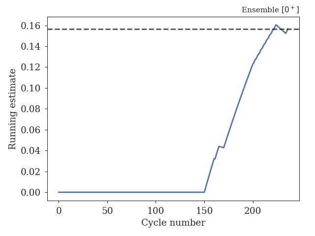
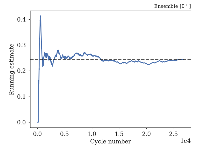
Has the running average flattened? Look at overall-prun and the per-ensemble NNN_prun. A curve still trending at the right edge means the estimate is still moving; the run needs more cycles.

The two below are the same ensemble of the same system, at 200 and at 20000 cycles. On the left the estimate sits at zero until cycle 150 – nothing had crossed yet – and is then climbing steeply when the run ends: whatever number that run reports is the value the curve happened to have reached. On the right it swings wildly for the first few thousand cycles and then settles onto 0.242 and stays there. That settling is what “converged” looks like.
Has the block-error curve reached a plateau? In overall-err and NNN_perror, a curve still rising at the largest block length means the quoted error is an underestimate – the samples are more correlated than the run is long.
Is the matched probability smooth? Kinks at interface positions in matched-probability mean neighbouring ensembles do not agree in their overlap region. A healthy one falls smoothly through orders of magnitude, with the interfaces (dashed) spread evenly along the decay – here from 1 to about $4 \times 10^{-7}$, the crossing probability the run reports. It flattens past the last interface because nothing beyond it was sampled.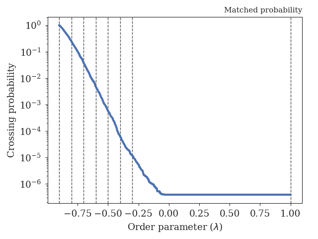
Are the per-ensemble numbers sane? Crossing probabilities of exactly 0 or exactly 1, acceptance ratios near zero, or path-length distributions piled up against maxlength all point at a badly configured ensemble rather than at a merely short run.

If a run fails only test 2 or 3, it needs more cycles. If it fails 4 or 5, more cycles will not help on their own: the interfaces are probably placed too far apart, or the move set does not suit the system.

A worked example: the same simulation, short and long ¶

The clearest way to learn the difference is to read one system’s report twice. Both runs below are the shipped 1D double-well RETIS example, unchanged except for [simulation] steps.

Too short: 200 cycles ¶

* The crossing probability:
  P_cross = 0.000000000e+00  ±  nan %
* The initial flux (unit: 1/reduced):
  f_A = 0.417660720  ±  6.431378533 %
* The rate constant (unit: 1/reduced):
  k_AB = 0.000000000e+00  ±  nan %

This looks alarming and is merely short. Nothing is broken: the flux is measured perfectly well, because it only needs the innermost ensemble. But in 200 cycles no path ever reached the outermost interface, so the crossing probability is exactly zero, and the rate – their product – with it. The nan is the honest report of an error that cannot be formed from zero successes, not a numerical fault.

The tell that this is a short run and not a broken one is that everything else looks healthy: the per-ensemble table of the same run has shooting acceptance ratios between 0.5 and 0.9, and sensible path lengths. Test 1 fails; tests 4 and 5 pass.

Long enough: 20000 cycles ¶

* The crossing probability:
  P_cross = 3.908476360e-07  ±  53.824318315 %
* The initial flux (unit: 1/reduced):
  f_A = 0.271443162  ±  2.832354761 %
* The rate constant (unit: 1/reduced):
  k_AB = 1.060929183e-07  ±  53.898789185 %

Now there is a rate. Note what did not change much: the flux, which was already well determined after 200 cycles (2.8 % error here). All the difficulty is in the crossing probability, and it is worth seeing why:

| Ensemble |   Pcross   |   Error    | Rel. error (%) |
|  [0^+]   |  0.244074  |  0.017055  |    6.987693    |
|  [1^+]   |  0.155206  |  0.018709  |   12.054258    |
|  [2^+]   |  0.124862  |  0.020380  |   16.322180    |
|  [3^+]   |  0.124981  |  0.022884  |   18.309615    |
|  [4^+]   |  0.106953  |  0.027190  |   25.422839    |
|  [5^+]   |  0.188040  |  0.031766  |   16.893095    |
|  [6^+]   |  0.032874  |  0.011243  |   34.198995    |

Each ensemble measures a conditional probability of order 0.1, none of them alarming on its own. The overall crossing probability is their product – which is how a rate of $10^{-7}$ is obtained from simulations that never wait $10^{7}$ steps for anything – and the relative errors compound along the chain, from 7 % at the innermost interface to 34 % at the outermost, giving the 54 % on the final result.

So this run has converged in the sense that matters least and most. It has converged enough to produce a rate, which the 200-cycle run could not; it has not converged to a precise one. If you need better than a factor of two, this system needs more cycles, more interfaces in the outer region, or both. Reading the error is not optional.

A second system: water-dimer dissociation with GROMACS ¶

The double well above is a one-particle toy. The same report on a real MD engine – the shipped water-dimer RETIS example, GROMACS at 250 K, 2000 cycles, order parameter the O–O distance – reads:

* The crossing probability:
  P_cross = 0.116483662  ±  33.757375544 %
* The initial flux (unit: 1/gromacs):
  f_A = 0.155524126  ±  24.403500782 %
* The rate constant (unit: 1/gromacs):
  k_AB = 1.811601973e-02  ±  41.654426584 %

The striking difference is the size of the answer: a crossing probability of 0.12 against the double well’s $4 \times 10^{-7}$. Breaking a water dimer is not a rare event on this order parameter – it is barely activated – so the per-ensemble probabilities run the other way:

| Ensemble |   Pcross   |   Error    | Rel. error (%) |
|  [0^+]   |  0.428929  |  0.121031  |   28.216993    |
|  [1^+]   |  0.558257  |  0.073001  |   13.076596    |
|  [2^+]   |  0.722222  |  0.081805  |   11.326792    |
|  [3^+]   |  0.882557  |  0.043049  |    4.877726    |
|  [4^+]   |  0.878774  |  0.030353  |    3.453983    |
|  [5^+]   |  0.929374  |  0.019230  |    2.069189    |
|  [6^+]   |  0.934468  |  0.018839  |    2.016036    |

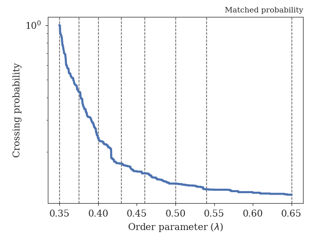
The water dimer's matched crossing probability, falling by less than two orders of magnitude.

Put that beside the double well’s curve above and the difference is the whole story: this one spans well under two orders of magnitude, and most of the drop happens between the first two interfaces. They rise outward, 0.43 to 0.93, where the double well’s fell. Once the dimer is stretched past the inner interfaces it comes apart almost every time, so the outer ensembles are easy and the whole difficulty sits at the first interface – which is also where the largest relative error is. Read that as a design signal: this interface set is finer than this system needs at the outside and too coarse at the inside.

The acceptance table tells the same story from the sampling side:

| Ensemble | TIS cycles | Shoot acc. ratio | Swap acc. ratio |  Exchange  |
|  [0^-]   |    1998    |     0.617647     |    0.978632     |  0.000000  |
|  [0^+]   |    7074    |     0.689922     |    0.978632     |  0.242415  |
|  [1^+]   |    9798    |     0.600000     |      n/a        |  0.445224  |
|  [2^+]   |   10054    |     0.460630     |      n/a        |  0.597915  |
|  [3^+]   |   10394    |     0.351852     |      n/a        |  0.711665  |
|  [4^+]   |    9870    |     0.274510     |      n/a        |  0.738265  |
|  [5^+]   |    9178    |     0.178862     |      n/a        |  0.758949  |
|  [6^+]   |    8636    |     0.093496     |      n/a        |  0.757857  |

Shooting acceptance falls steeply outward, 0.69 down to 0.09 – an external engine on a floppy molecule is far harder to shoot in than a Langevin particle in a smooth well, where the same column only fell to 0.64. An acceptance below 0.1 in the outermost ensemble is the number to act on: it says most of the work spent there is thrown away, and that the interfaces are too widely spaced at the outside.

Note also that Exchange rises outward here (0.24 to 0.76) while acceptance falls. That is the infinite-swapping machinery doing its job: where shooting struggles, the ensembles lean more on exchanging occupancy with their neighbours.

Note

The engine unit shows in the report (1/gromacs), because the rate carries whatever time unit the engine works in. Compare rates only after converting to a physical unit.

The health check ¶

The per-ensemble table of the long run is what a well-behaved RETIS simulation looks like:

| Ensemble | TIS cycles | Shoot acc. ratio | Swap acc. ratio | Avg. path length |
|  [0^-]   |   19998    |     0.808360     |    1.000000     |    1.5051e+03    |
|  [0^+]   |   26839    |     0.918100     |    1.000000     |    340.941287    |
|  [1^+]   |   29581    |     0.810756     |      n/a        |    507.382453    |
|  [2^+]   |   27511    |     0.718249     |      n/a        |    608.313264    |
|  [3^+]   |   26428    |     0.686131     |      n/a        |    713.262891    |
|  [4^+]   |   26173    |     0.682670     |      n/a        |    819.305071    |
|  [5^+]   |   26499    |     0.671490     |      n/a        |    954.391600    |
|  [6^+]   |   24253    |     0.636364     |      n/a        |    1.1479e+03    |

Two trends are the signature of a healthy run, and both are visible:

Acceptance falls outwards, 0.92 down to 0.64. Outer ensembles ask more of a trajectory, so more trials are rejected. A flat column – and especially a column of exactly 1.000000 – would mean the rejections are not being counted, not that the sampling is perfect.
Paths grow longer outwards, 341 up to 1148 frames, because a path has further to travel before it can return. Lengths that stop growing, or that pile up at maxlength, mean trajectories are being truncated.

The swap column reads n/a from [1^+] outwards by design, as explained above: only the zero swap is an accept/reject move.