Both rates in one run (biretis)

In this example, you will compute the rate constant of a transition in both directions, \(k_{AB}\) and \(k_{BA}\), and the equilibrium constant \(K = k_{AB} / k_{BA}\), with one bidirectional RETIS simulation (the biretis task). A retis simulation gives the rate of one direction, and the rate of the other direction needs a second retis simulation, which samples the paths over the barrier again. A biretis simulation samples those paths once, for both directions.

The system is the double well of the RETIS example, made asymmetric: \(V_{\text{pot}} = x^4 - 2 (x - 0.03)^2\). State A, the well at \(x \approx -1\), is deeper than state B, the well at \(x \approx 1\), so the transition from B to A is the faster one.

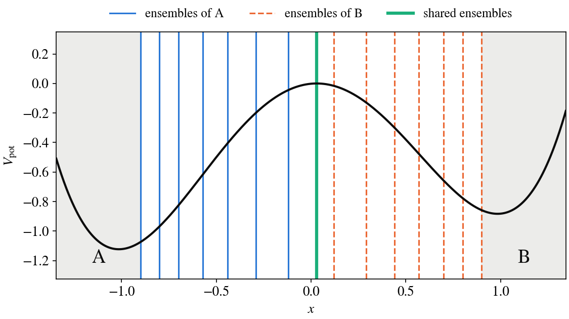
Fig. 31 The potential and the ensembles of the example. The ensembles of A (solid) climb from \(\lambda_A = -0.9\), the ensembles of B (dashed) descend from \(\lambda_B = 0.9\), and the two meet in one shared ensemble at the top of the barrier, \(x = 0.03\). The script plot_layout.py of the tutorial draws this figure from the input.

Verification status: smoke – see Tutorial map.

Tutorial quick start

• Best starting point: examples/tutorials/path_sampling/internal/1D-double-well/biretis/.

• Edit first: biretis.toml, for the interfaces of the two states and shared; python plot_layout.py draws them on the potential, into layout.png.

• Run: pyretis run -i biretis.toml -p.

• Analyse: pyretis analyse -i biretis.toml -skipb 2000, which leaves out the first 2000 cycles.

• Compare: python brute_force_rates.py computes the rates of the same dynamics by brute force, from the transitions of long plain trajectories, in a few minutes.

• Expected output: the ensemble directories 000 to 016, pyretis.log, output.toml and, after the analysis, report/biretis_report.txt.

How one run samples both directions

A path that starts in A is a path of state A, and a path that starts in B is a path of state B. The run samples two ladders of ensembles:

• the ensembles of A hold the paths that start in A and cross an interface of A on their way up from \(\lambda_A\). With the \([0^-]\) ensemble of A, which gives the flux out of A, they give the rate from A to B, as a retis run does;

• the ensembles of B hold the paths that start in B and cross an interface of B on their way down from \(\lambda_B\). With the \([0^-]\) ensemble of B, they give the rate from B to A.

A reactive path from A to B is, run backwards, a reactive path from B to A. The shared ensemble at the top of the barrier holds the paths of both states that cross it, and a time reversal there turns the one into the other: the run samples each reactive path once and counts it for both rates.

Setting up the simulation

The simulation section gives the task, the number of cycles and the interfaces of the two states:

[simulation]
task = "biretis"
steps = 20000
interfaces = [-0.9, -0.8, -0.7, -0.57, -0.44, -0.29, -0.12, 0.03, 0.9]
interfaces_b = [0.9, 0.8, 0.7, 0.57, 0.44, 0.29, 0.12, 0.03, -0.9]
shared = 1

• interfaces are the interfaces of state A, as for retis: ascending from \(\lambda_A = -0.9\) to \(\lambda_B = 0.9\).

• interfaces_b are the interfaces of state B, descending from \(\lambda_B\) to \(\lambda_A\).

• shared = 1 pairs the last interface of each list before the other state, 0.03 in both lists, into one shared ensemble.

The other sections set one particle in one dimension, the Langevin engine in its high-friction limit (gamma = 1.0) at the temperature 0.2, and the position of the particle as the order parameter. The potential is the tilted double well:

potential = [
    { class = "DoubleWell", a = 1.0, b = 2.0, c = 0.03 },
]

and one move out of ten is a time reversal (freq):

[tis]
# A time reversal in a shared ensemble turns a path from A to B into the
# path from B to A it is in reverse.
freq = 0.1
maxlength = 50000
allowmaxlength = false
zero_momentum = false

Show/hide the full input file »

# Bidirectional RETIS: the rates of A -> B and of B -> A in one run.
#
# An asymmetric double well, V = x^4 - 2 (x - 0.03)^2, with Brownian
# dynamics at kB T = 0.2. State A (x <= -0.9) is the deeper well, so the
# rate from B to A is the larger one; K = k_AB / k_BA is about 0.31.
#
# The A ladder climbs from lambda_A = -0.9 and the B ladder descends from
# lambda_B = 0.9. They meet at 0.03, the top of the barrier, where a path
# that has come from A and one that has come from B are equally likely to
# go on to the other state. The last interface of each list before the
# other state is that meeting interface, and shared = 1 pairs the two
# into one shared ensemble, which holds the paths of both states.
potential = [
    { class = "DoubleWell", a = 1.0, b = 2.0, c = 0.03 },
]

[simulation]
task = "biretis"
steps = 20000
interfaces = [-0.9, -0.8, -0.7, -0.57, -0.44, -0.29, -0.12, 0.03, 0.9]
interfaces_b = [0.9, 0.8, 0.7, 0.57, 0.44, 0.29, 0.12, 0.03, -0.9]
shared = 1

[system]
units = "reduced"
dimensions = 1
temperature = 0.2

[engine]
class = "Langevin"
timestep = 0.002
gamma = 1.0
high_friction = true
seed = 0

[box]
periodic = [false]

[particles]
name = ["Ar"]
ptype = [0]

[particles.position]
input_file = "initial.xyz"

[particles.mass]
Ar = 1.0

[forcefield]
description = "1D asymmetric double well, Brownian dynamics"

[orderparameter]
class = "pyretis_position"
dim = "x"
index = 0
periodic = false

[output]
order-file = -1
energy-file = 0

[tis]
# A time reversal in a shared ensemble turns a path from A to B into the
# path from B to A it is in reverse.
freq = 0.1
maxlength = 50000
allowmaxlength = false
zero_momentum = false

Placing the interfaces

Each ladder is placed as for retis, with a local crossing probability of about 0.2 to 0.5 from one interface to the next. The shared ensemble works best where a path that has come from A and a path that has come from B are equally likely to go on to the other state: here, the top of the barrier. The analysis reports the fraction of the paths of the shared ensemble that start in A. It is close to one half in this example; a fraction below 0.2 or above 0.8 means that the shared ensemble sits too close to one of the states. The biretis task describes the placement for other systems.

Running and analysing

Run the simulation in a folder with the input and the initial configuration, biretis.toml and initial.xyz:

pyretis run -i biretis.toml -p

The run writes one directory per ensemble: 000 is the \([0^-]\) of A and 001 the \([0^-]\) of B, 002 to 008 are the ensembles of A, 009 to 015 those of B, and 016 is the shared ensemble. Analyse it with:

pyretis analyse -i biretis.toml -skipb 2000

The analysis writes report/biretis_report.txt, with the flux out of each state, the crossing probability of each state, the two rates, \(K\), their errors over five blocks of cycles, and the local crossing probability of each ensemble. -skipb 2000 leaves out the first 2000 cycles, which still depend on the kicked initial paths (see the results below).

Results

The tutorial input was run with 32 seeds ([simulation] seed from 1001 to 1032, with the seed of [engine] left out, since a run accepts it only when it equals [simulation] seed), for 20 000 cycles each. For comparison, each direction was computed with retis runs of the same interfaces and seeds: A to B with the interfaces of A, and B to A as the transition from A to B on the mirror image of the potential (c = -0.03, interfaces -0.9, -0.8, -0.7, -0.57, -0.44, -0.29, -0.12, -0.03, 0.9). The reference rates of this dynamics come from the script brute_force_rates.py of the tutorial, which follows 1000 walkers for \(10^6\) steps each, with the integrator of the Langevin engine, and counts 4611 transitions from A to B and 4644 from B to A: each brute-force rate has a standard error of 1.5 %.

Table 68 The mean over the runs, with its standard error, and the \(K\) of each route: the ratio of its two mean rates, with its standard error from the spread of the rates over the runs.

	biretis, 32 runs	retis, 32 + 32 runs	brute force
\(k_{AB}\)	\((3.36 \pm 0.17) \times 10^{-3}\)	\((3.29 \pm 0.13) \times 10^{-3}\)	\((3.03 \pm 0.05) \times 10^{-3}\)
\(k_{BA}\)	\((9.93 \pm 0.39) \times 10^{-3}\)	\((9.55 \pm 0.23) \times 10^{-3}\)	\((9.67 \pm 0.14) \times 10^{-3}\)
\(K\)	\(0.338 \pm 0.020\)	\(0.344 \pm 0.016\)	\(0.314 \pm 0.007\)
MD steps of one run	\(2.84 \times 10^{6}\)	\(2.80 \times 10^{6}\) (A to B) and \(3.05 \times 10^{6}\) (B to A)

The two routes agree with each other, and each agrees with the brute-force rates within two standard errors; for \(k_{AB}\) both routes lie above the brute-force rate, by 2.5 standard errors when the two are combined. The fluxes of the biretis runs, and the local crossing probabilities of all eight ensembles of each state, which brute force gives as well (among the excursions out of a state that cross an interface, the fraction that reach the next one), agree with it within 1.5 standard errors. In the shared ensemble, paths that start in A hold \(0.50 \pm 0.01\) of the occupancy.

These numbers use every cycle of the runs. The first cycles of a biretis run, which starts from kicked paths, raise both of its rates; those of the retis runs do not. With the first 2000 cycles of each run left out (pyretis analyse -i biretis.toml -skipb 2000), biretis gives \(k_{AB} = (3.31 \pm 0.18) \times 10^{-3}\), \(k_{BA} = (9.57 \pm 0.43) \times 10^{-3}\) and \(K = 0.345 \pm 0.023\), 2 % and 4 % lower rates, and the retis rates do not change.

One biretis run gives both rates and \(K\) for the MD steps of one retis run: half the steps of the two retis runs. Its results spread more from run to run: with 17 ensembles against 9, each ensemble is moved about half as often as in a retis run of as many cycles. Counted as the inverse of the relative variance of a run (its variance over its mean squared) times its MD steps, the efficiency of biretis is 1.2 for \(K\) relative to the two retis runs (0.8 with the first 2000 cycles left out), the same within the statistics of 32 runs, and, relative to the one retis run of that direction, 0.6 for \(k_{AB}\) (0.5) and 0.4 for \(k_{BA}\) (0.4). On this double well, biretis gives \(K\) as precisely as two retis runs for the same MD; for one rate alone, a retis run is the cheaper route.

On the symmetric double well (c = 0, mirror lists of interfaces), the mirror symmetry gives \(K = 1\), \(f_A = f_B\) and equal local crossing probabilities of the two states, without a brute-force reference. Three sets of runs were tested this way, each with its first cycles left out:

• underdamped Langevin dynamics (high_friction = false, gamma = 0.3), one shared ensemble at 0.0, 16 runs: \(K = 0.90 \pm 0.17\), \(f_A - f_B\) of \((-1.1 \pm 1.6)\) % of the flux, the A-start fraction of the shared ensemble \(0.49 \pm 0.03\);

• one shared ensemble on the mirror pair -0.12 (A) and 0.12 (B), 16 runs: \(K = 0.83 \pm 0.10\), the A-start fraction \(0.51 \pm 0.03\);

• no shared ensemble (shared = 0), 8 runs: \(K = 0.83 \pm 0.30\).

In each set the local crossing probabilities of the two states agree (the \(\chi^2\) of the mirror pairs gives \(p = 0.07\), 0.30 and 0.97), and so do the fluxes; the largest deviation is \(f_A - f_B\) of the mirror pair, 2.2 standard errors.

Tested by

examples/run-tutorials.sh runs the tutorial for 20 cycles and analyses them (see Example test status).